Showing posts with label Linux. Show all posts
Showing posts with label Linux. Show all posts
Wednesday, February 22, 2012
In-memory database (inspired by 864GB of RAM for $12,000)
https://groups.google.com/forum/#!topic/nodejs/aqVYp5ABX_4
Tuesday, September 27, 2011
Monday, August 1, 2011
Nested RAID levels
(Cross-post from http://en.wikipedia.org/wiki/Nested_RAID_levels)
Nesting
When nesting RAID levels, a RAID type that provides redundancy is typically combined with RAID 0 to boost performance. With these configurations it is preferable to have RAID 0 on top and the redundant array at the bottom, because fewer disks need to be regenerated if a disk fails. (Thus, RAID 1+0 is preferable to RAID 0+1 but the administrative advantages of "splitting the mirror" of RAID 1 are lost. It should be noted, however, that the on-disk layout of blocks for RAID 1+0 and RAID 0+1 setups are identical so these limitations are purely in the software).
A RAID 0+1 (also called RAID 01), is a RAID level used for both replicating and sharing data among disks.[3] The minimum number of disks required to implement this level of RAID is 3 (first, even numbered chunks on all disks are built – like in RAID 0 – and then every odd chunk number is mirrored with the next higher even neighbour) but it is more common to use a minimum of 4 disks. The difference between RAID 0+1 and RAID 1+0 is the location of each RAID system — RAID 0+1 is a mirror of stripes although some manufacturers (e.g. Digital/Compaq/HP) use RAID 0+1 to describe striped mirrors, consequently this useage is now deprecated so that RAID 0+1 and RAID1+0 are replaced by RAID10 whose definition correctly describes the correct and safe layout ie striped mirrors. The usable capacity of a RAID 0+1 array is , where N is the total number of drives (must be even) in the array and Smin is the capacity of the smallest drive in the array.

The maximum storage space here is 360 GB, spread across two arrays. The advantage is that when a hard drive fails in one of the level 0 arrays, the missing data can be transferred from the other array. However, adding an extra hard drive to one stripe requires you to add an additional hard drive to the other stripes to balance out storage among the arrays.
It is not as robust as RAID 10 and cannot tolerate two simultaneous disk failures. When 1 disk fails, the RAID 0 array that it is in will fail also. The RAID 10 array will continue to work on the remaining RAID 0 array. If a disk from that array fails before the first failing disk has been replaced, the data will be lost. That is, once a single disk fails, each of the mechanisms in the other stripe is single point of failure. Also, once the single failed mechanism is replaced, in order to rebuild its data all the disks in the array must participate in the rebuild.
The exception to this is if all the disks are hooked up to the same RAID controller in which case the controller can do the same error recovery as RAID 10 as it can still access the functional disks in each RAID 0 set. If you compare the diagrams between RAID 0+1 and RAID 10 and ignore the lines above the disks you will see that all that's different is that the disks are swapped around. If the controller has a direct link to each disk it can do the same. In this one case there is no difference between RAID 0+1 and RAID 10.
Additionally, bit error correction technologies have not kept up with rapidly rising drive capacities, resulting in higher risks of encountering media errors. In the case where a failed drive is not replaced in a RAID 0+1 configuration, a single uncorrectable media error occurring on the mirrored hard drive would result in data loss.
Given these increasing risks with RAID 0+1, many business and mission critical enterprise environments are beginning to evaluate more fault tolerant RAID setups, both RAID 10 and formats such as RAID 5 and RAID 6 that provide a smaller improvement than RAID 10 by adding underlying disk parity, but reduce overall cost. Among the more promising are hybrid approaches such as RAID 51 (mirroring above single parity) or RAID 61 (mirroring above dual parity) although neither of these delivers the reliability of the more expensive option of using RAID 10 with three way mirrors.

A RAID 1+0, sometimes called RAID 1&0 or RAID 10, is similar to a RAID 0+1 with exception that the RAID levels used are reversed — RAID 10 is a stripe of mirrors.[3]
Laptop and motherboard makers were expected to routinely include two-disk RAID 10 as options on their products by 2011[citation needed] and even configure some OEM versions of operating systems with this as a default[citation needed]. Among Linux users it has become extremely common.
Another use for these configurations is to continue to use slower disk interfaces in NAS or low-end RAIDs/SAS (notably SATA-II at 300 MB/s or 3 Gbit/s) rather than replace them with faster ones (USB-3 at 480 MB/s or 4.8 Gbit/s, SATA-III at 600 MB/s or 6 Gbit/s, PCIe x4 at 730 MB/s, PCIe x8 at 1460 MB/s, etc.). A pair of identical SATA-II disks with any of hybrid SSD, OS caching to a SSD or a large software write cache, could be expected to achieve performance identical to SATA-III. Three or four could achieve at least read performance similar to PCIe x8 or striped SATA-III if properly configured to minimize seek time (predictable offsets, redundant copies of most accessed data).

More typically, larger arrays of disks are combined for professional applications. In high end configurations, enterprise storage experts expected PCIe and SAS storage to dominate and eventually replace interfaces designed for spinning metal[6] and for these interfaces to become further integrated with Ethernet and network storage suggesting that rarely-accessed data stripes could often be located over networks and that very large arrays using protocols like iSCSI would become more common. Below is an example where three collections of 120 GB level 1 arrays are striped together to make 360 GB of total storage space:
It is the preferable RAID level for I/O-intensive applications such as database, email, and web servers, as well as for any other use requiring high disk performance.[10]
, where N is the total number of drives in the array and Smin is the capacity of the smallest drive in the array.

RAID level 0+3 or RAID level 03 is a dedicated parity array across striped disks. Each block of data at the RAID 3 level is broken up amongst RAID 0 arrays where the smaller pieces are striped across disks.

RAID level 30 is also known as striping of dedicated parity arrays. It is a combination of RAID level 3 and RAID level 0. RAID 30 provides high data transfer rates, combined with high data reliability. RAID 30 is best implemented on two RAID 3 disk arrays with data striped across both disk arrays. RAID 30 breaks up data into smaller blocks, and then stripes the blocks of data to each RAID 3 RAID set. RAID 3 breaks up data into smaller blocks, calculates parity by performing an Exclusive OR on the blocks, and then writes the blocks to all but one drive in the array. The parity bit created using the Exclusive OR is then written to the last drive in each RAID 3 array. The size of each block is determined by the stripe size parameter, which is set when the RAID is created.
One drive from each of the underlying RAID 3 sets can fail. Until the failed drives are replaced the other drives in the sets that suffered such a failure are a single point of failure for the entire RAID 30 array. In other words, if one of those drives fails, all data stored in the entire array is lost. The time spent in recovery (detecting and responding to a drive failure, and the rebuild process to the newly inserted drive) represents a period of vulnerability to the RAID set.

The failure characteristics are identical to RAID 10: all but one drive from each RAID 1 set could fail without loss of data. However, the remaining disk from the RAID 1 becomes a single point of failure for the already degraded array. Often the top level stripe is done in software. Some vendors call the top level stripe a MetaLun (Logical Unit Number (LUN)), or a Soft Stripe.
The major benefits of RAID 100 (and plaid RAID in general) over single-level RAID is spreading the load across multiple RAID controllers, giving better random read performance and mitigating hotspot risk on the array. For these reasons, RAID 100 is often the best choice for very large databases, where the hardware RAID controllers limit the number of physical disks allowed in each standard array. Implementing nested RAID levels allows virtually limitless spindle counts in a single logical volume.

A RAID 50 combines the straight block-level striping of RAID 0 with the distributed parity of RAID 5.[3] This is a RAID 0 array striped across RAID 5 elements. It requires at least 6 drives.
Below is an example where three collections of 240 GB RAID 5s are striped together to make 720 GB of total storage space:
One drive from each of the RAID 5 sets could fail without loss of data. However, if the failed drive is not replaced, the remaining drives in that set then become a single point of failure for the entire array. If one of those drives fails, all data stored in the entire array is lost. The time spent in recovery (detecting and responding to a drive failure, and the rebuild process to the newly inserted drive) represents a period of vulnerability to the RAID set.
In the example below, datasets may be striped across both RAID sets. A dataset with 5 blocks would have 3 blocks written to the first RAID set, and the next 2 blocks written to RAID set 2.

The configuration of the RAID sets will impact the overall fault tolerance. A construction of three seven-drive RAID 5 sets has higher capacity and storage efficiency, but can only tolerate three maximum potential drive failures. Because the reliability of the system depends on quick replacement of the bad drive so the array can rebuild, it is common to construct three six-drive RAID 5 sets each with a hot spare that can immediately start rebuilding the array on failure. This does not address the issue that the array is put under maximum strain reading every bit to rebuild the array precisely at the time when it is most vulnerable. A construction of seven three-drive RAID 5 sets can handle as many as seven drive failures but has lower capacity and storage efficiency.
RAID 50 improves upon the performance of RAID 5 particularly during writes, and provides better fault tolerance than a single RAID level does. This level is recommended for applications that require high fault tolerance, capacity and random positioning performance.
As the number of drives in a RAID set increases, and the capacity of the drives increase, this impacts the fault-recovery time correspondingly as the interval for rebuilding the RAID set increases.

A RAID 51 or RAID 5+1 is an array that consists of two RAID 5's that are mirrors of each other. Generally this configuration is used so that each RAID 5 resides on a separate controller. In this configuration reads and writes are balanced across both RAID 5s. Some controllers support RAID 51 across multiple channels and cards with hinting to keep the different slices synchronized. However a RAID 51 can also be accomplished using a layered RAID technique. In this configuration, the two RAID 5's have no idea that they are mirrors of each other and the RAID 1 has no idea that its underlying disks are RAID 5's. This configuration can sustain the failure of all disks in either of the arrays, plus up to one additional disk from the other array before suffering data loss. The maximum amount of space of a RAID 51 is (N) where N is the size of an individual RAID 5 set.
Below is an example where two collections of 240 GB RAID 6s are striped together to make 480 GB of total storage space:

As it is based on RAID 6, two disks from each of the RAID 6 sets could fail without loss of data. Also failures while a single disk is rebuilding in one RAID 6 set will not lead to data loss. RAID 60 has improved fault tolerance, any two drives can fail without data loss and up to four total as long as it is only two from each RAID 6 sub-array.
Striping helps to increase capacity and performance without adding disks to each RAID 6 set (which would decrease data availability and could impact performance). RAID 60 improves upon the performance of RAID 6. Despite the fact that RAID 60 is slightly slower than RAID 50 in terms of writes due to the added overhead of more parity calculations, when data security is concerned this performance drop may be negligible.
m - Bottom Level Division

Nesting
| This section does not cite any references or sources. Please help improve this section by adding citations to reliable sources. Unsourced material may be challenged and removed. (September 2010) |
When nesting RAID levels, a RAID type that provides redundancy is typically combined with RAID 0 to boost performance. With these configurations it is preferable to have RAID 0 on top and the redundant array at the bottom, because fewer disks need to be regenerated if a disk fails. (Thus, RAID 1+0 is preferable to RAID 0+1 but the administrative advantages of "splitting the mirror" of RAID 1 are lost. It should be noted, however, that the on-disk layout of blocks for RAID 1+0 and RAID 0+1 setups are identical so these limitations are purely in the software).
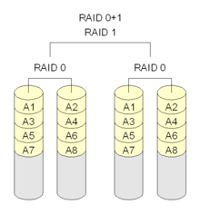
RAID 0+1

Typical RAID 0+1 setup.
A RAID 0+1 (also called RAID 01), is a RAID level used for both replicating and sharing data among disks.[3] The minimum number of disks required to implement this level of RAID is 3 (first, even numbered chunks on all disks are built – like in RAID 0 – and then every odd chunk number is mirrored with the next higher even neighbour) but it is more common to use a minimum of 4 disks. The difference between RAID 0+1 and RAID 1+0 is the location of each RAID system — RAID 0+1 is a mirror of stripes although some manufacturers (e.g. Digital/Compaq/HP) use RAID 0+1 to describe striped mirrors, consequently this useage is now deprecated so that RAID 0+1 and RAID1+0 are replaced by RAID10 whose definition correctly describes the correct and safe layout ie striped mirrors. The usable capacity of a RAID 0+1 array is
, where N is the total number of drives (must be even) in the array and Smin is the capacity of the smallest drive in the array.Six-drive RAID 0+1
Consider an example of RAID 0+1: six 120 GB drives need to be set up on a RAID 0+1. Below is an example where two 360 GB level 0 arrays are mirrored, creating 360 GB of total storage space:
Note: A1, A2, et cetera each represent one data block; each column represents one disk.
The maximum storage space here is 360 GB, spread across two arrays. The advantage is that when a hard drive fails in one of the level 0 arrays, the missing data can be transferred from the other array. However, adding an extra hard drive to one stripe requires you to add an additional hard drive to the other stripes to balance out storage among the arrays.
It is not as robust as RAID 10 and cannot tolerate two simultaneous disk failures. When 1 disk fails, the RAID 0 array that it is in will fail also. The RAID 10 array will continue to work on the remaining RAID 0 array. If a disk from that array fails before the first failing disk has been replaced, the data will be lost. That is, once a single disk fails, each of the mechanisms in the other stripe is single point of failure. Also, once the single failed mechanism is replaced, in order to rebuild its data all the disks in the array must participate in the rebuild.
The exception to this is if all the disks are hooked up to the same RAID controller in which case the controller can do the same error recovery as RAID 10 as it can still access the functional disks in each RAID 0 set. If you compare the diagrams between RAID 0+1 and RAID 10 and ignore the lines above the disks you will see that all that's different is that the disks are swapped around. If the controller has a direct link to each disk it can do the same. In this one case there is no difference between RAID 0+1 and RAID 10.
Additionally, bit error correction technologies have not kept up with rapidly rising drive capacities, resulting in higher risks of encountering media errors. In the case where a failed drive is not replaced in a RAID 0+1 configuration, a single uncorrectable media error occurring on the mirrored hard drive would result in data loss.
Given these increasing risks with RAID 0+1, many business and mission critical enterprise environments are beginning to evaluate more fault tolerant RAID setups, both RAID 10 and formats such as RAID 5 and RAID 6 that provide a smaller improvement than RAID 10 by adding underlying disk parity, but reduce overall cost. Among the more promising are hybrid approaches such as RAID 51 (mirroring above single parity) or RAID 61 (mirroring above dual parity) although neither of these delivers the reliability of the more expensive option of using RAID 10 with three way mirrors.
RAID 1 + 0

Typical RAID 1+0 setup.
Near versus far, advantages for bootable RAID
A nonstandard definition of "RAID 10" was created for the Linux MD driver[4] ; RAID 10 as recognized by the storage industry association and as generally implemented by RAID controllers is a RAID 0 array of mirrors (which may be two way or three way mirrors) [5] and requires a minimum of 4 drives. Linux "RAID 10" can be implemented with as few as two disks. Implementations supporting two disks such as Linux RAID 10[4] offer a choice of layouts, including one in which copies of a block of data are "near" each other or at the same address on different devices or predictably offset: Each disk access is split into full-speed disk accesses to different drives, yielding read and write performance like RAID 0 but without necessarily guaranteeing every stripe is on both drives. Another layout uses "a more RAID 0 like arrangement over the first half of all drives, and then a second copy in a similar layout over the second half of all drives - making sure that all copies of a block are on different drives." This has high read performance because only one of the two read locations must be found on each access, but writing requires more head seeking as two write locations must be found. Very predictable offsets minimize the seeking in either configuration. "Far" configurations may be exceptionally useful for Hybrid SSD with huge caches of 4 GB (compared to the more typical 64 MB of spinning platters in 2010) and by 2011 64 GB (as this level of storage exists now on one single chip). They may also be useful for those small pure SSD bootable RAIDs which are not reliably attached to network backup and so must maintain data for hours or days, but which are quite sensitive to the cost, power and complexity of more than two disks. Write access for SSDs is extremely fast so the multiple access become less of a problem with speed: At PCIe x4 SSD speeds, the theoretical maximum of 730 MB/s is already more than double the theoretical maximum of SATA-II at 300 MB/s.Laptop and motherboard makers were expected to routinely include two-disk RAID 10 as options on their products by 2011[citation needed] and even configure some OEM versions of operating systems with this as a default[citation needed]. Among Linux users it has become extremely common.
Another use for these configurations is to continue to use slower disk interfaces in NAS or low-end RAIDs/SAS (notably SATA-II at 300 MB/s or 3 Gbit/s) rather than replace them with faster ones (USB-3 at 480 MB/s or 4.8 Gbit/s, SATA-III at 600 MB/s or 6 Gbit/s, PCIe x4 at 730 MB/s, PCIe x8 at 1460 MB/s, etc.). A pair of identical SATA-II disks with any of hybrid SSD, OS caching to a SSD or a large software write cache, could be expected to achieve performance identical to SATA-III. Three or four could achieve at least read performance similar to PCIe x8 or striped SATA-III if properly configured to minimize seek time (predictable offsets, redundant copies of most accessed data).
Examples

Note: A1, A2, et cetera each represent one data block; each column represents one disk.
More typically, larger arrays of disks are combined for professional applications. In high end configurations, enterprise storage experts expected PCIe and SAS storage to dominate and eventually replace interfaces designed for spinning metal[6] and for these interfaces to become further integrated with Ethernet and network storage suggesting that rarely-accessed data stripes could often be located over networks and that very large arrays using protocols like iSCSI would become more common. Below is an example where three collections of 120 GB level 1 arrays are striped together to make 360 GB of total storage space:
Redundancy and data-loss recovery capability
All but one drive from each RAID 1 set could fail without damaging the data. However, if the failed drive is not replaced, the single working hard drive in the set then becomes a single point of failure for the entire array. If that single hard drive then fails, all data stored in the entire array is lost. As is the case with RAID 0+1, if a failed drive is not replaced in a RAID 10 configuration then a single uncorrectable media error occurring on the mirrored hard drive would result in data loss. Some RAID 10 vendors address this problem by supporting a "hot spare" drive, which automatically replaces and rebuilds a failed drive in the array.Performance (speed)
According to manufacturer specifications[7] and official independent benchmarks,[8][9] in most cases RAID 10 provides better throughput and latency than all other RAID levels except RAID 0 (which wins in throughput).It is the preferable RAID level for I/O-intensive applications such as database, email, and web servers, as well as for any other use requiring high disk performance.[10]
Efficiency (potential waste of storage)
The usable capacity of a RAID 10 array is, where N is the total number of drives in the array and Smin is the capacity of the smallest drive in the array.Implementation
The Linux kernel RAID 10 implementation (from version 2.6.9 and onwards) is not nested. The mirroring and striping is done in one process. Only certain layouts are standard RAID 10.[4] See also the Linux MD RAID 10 and RAID 1.5 sections in the Non-standard RAID article for details.RAID 0+3 and 3+0
| This section does not cite any references or sources. Please help improve this section by adding citations to reliable sources. Unsourced material may be challenged and removed. (September 2010) |
RAID 0+3

Diagram of a 0+3 array
RAID level 0+3 or RAID level 03 is a dedicated parity array across striped disks. Each block of data at the RAID 3 level is broken up amongst RAID 0 arrays where the smaller pieces are striped across disks.
RAID 30

Diagram of a 3+0 array
RAID level 30 is also known as striping of dedicated parity arrays. It is a combination of RAID level 3 and RAID level 0. RAID 30 provides high data transfer rates, combined with high data reliability. RAID 30 is best implemented on two RAID 3 disk arrays with data striped across both disk arrays. RAID 30 breaks up data into smaller blocks, and then stripes the blocks of data to each RAID 3 RAID set. RAID 3 breaks up data into smaller blocks, calculates parity by performing an Exclusive OR on the blocks, and then writes the blocks to all but one drive in the array. The parity bit created using the Exclusive OR is then written to the last drive in each RAID 3 array. The size of each block is determined by the stripe size parameter, which is set when the RAID is created.
One drive from each of the underlying RAID 3 sets can fail. Until the failed drives are replaced the other drives in the sets that suffered such a failure are a single point of failure for the entire RAID 30 array. In other words, if one of those drives fails, all data stored in the entire array is lost. The time spent in recovery (detecting and responding to a drive failure, and the rebuild process to the newly inserted drive) represents a period of vulnerability to the RAID set.
RAID 100 (RAID 1+0+0)
A RAID 100, sometimes also called RAID 10+0, is a stripe of RAID 10s. This is logically equivalent to a wider RAID 10 array, but is generally implemented using software RAID 0 over hardware RAID 10. Being "striped two ways", RAID 100 is described as a "plaid RAID".[11] Below is an example in which two sets of two 120 GB RAID 1 arrays are striped and re-striped to make 480 GB of total storage space:
Representative RAID-100 Setup.
(Note: A1, B1, et cetera each represent one data sector; each column represents one disk.)
(Note: A1, B1, et cetera each represent one data sector; each column represents one disk.)
The major benefits of RAID 100 (and plaid RAID in general) over single-level RAID is spreading the load across multiple RAID controllers, giving better random read performance and mitigating hotspot risk on the array. For these reasons, RAID 100 is often the best choice for very large databases, where the hardware RAID controllers limit the number of physical disks allowed in each standard array. Implementing nested RAID levels allows virtually limitless spindle counts in a single logical volume.
RAID 50 (RAID 5+0)

Representative RAID-50 Setup.
(Note: A1, B1, et cetera each represent one data block; each column represents one disk; Ap, Bp, et cetera each represent parity information for each distinct RAID 5 and may represent different values across the RAID 5 (that is, Ap for A1 and A2 can differ from Ap for A3 and A4).)
(Note: A1, B1, et cetera each represent one data block; each column represents one disk; Ap, Bp, et cetera each represent parity information for each distinct RAID 5 and may represent different values across the RAID 5 (that is, Ap for A1 and A2 can differ from Ap for A3 and A4).)
Below is an example where three collections of 240 GB RAID 5s are striped together to make 720 GB of total storage space:
One drive from each of the RAID 5 sets could fail without loss of data. However, if the failed drive is not replaced, the remaining drives in that set then become a single point of failure for the entire array. If one of those drives fails, all data stored in the entire array is lost. The time spent in recovery (detecting and responding to a drive failure, and the rebuild process to the newly inserted drive) represents a period of vulnerability to the RAID set.
In the example below, datasets may be striped across both RAID sets. A dataset with 5 blocks would have 3 blocks written to the first RAID set, and the next 2 blocks written to RAID set 2.

RAID-50 Setup consisting of two sets of four drives each.
RAID 50 improves upon the performance of RAID 5 particularly during writes, and provides better fault tolerance than a single RAID level does. This level is recommended for applications that require high fault tolerance, capacity and random positioning performance.
As the number of drives in a RAID set increases, and the capacity of the drives increase, this impacts the fault-recovery time correspondingly as the interval for rebuilding the RAID set increases.
RAID 51

Diagram of a RAID 51 setup.
RAID 05 (RAID 0+5)
A RAID 0 + 5 consists of several RAID 0's (a minimum of three) that are grouped into a single RAID 5 set. The total capacity is (N-1) where N is total number of RAID 0's that make up the RAID 5. This configuration is not generally used in production systems.RAID 53
Note that RAID 53 is typically used as a name for RAID 30 or 0+3.[12]RAID 60 (RAID 6+0)
A RAID 60 combines the straight block-level striping of RAID 0 with the distributed double parity of RAID 6. That is, a RAID 0 array striped across RAID 6 elements. It requires at least 8 disks.[3]Below is an example where two collections of 240 GB RAID 6s are striped together to make 480 GB of total storage space:

RAID-60 (RAID 6+0) Setup consisting of two sets of four drives each.
Striping helps to increase capacity and performance without adding disks to each RAID 6 set (which would decrease data availability and could impact performance). RAID 60 improves upon the performance of RAID 6. Despite the fact that RAID 60 is slightly slower than RAID 50 in terms of writes due to the added overhead of more parity calculations, when data security is concerned this performance drop may be negligible.
Nested RAID comparison
n - Top Level Divisionm - Bottom Level Division

- ^ Delmar, Michael Graves (2003). "Data Recovery and Fault Tolerance". The Complete Guide to Networking and Network+. Cengage Learning. p. 448. ISBN 140183339X. http://books.google.com/books?id=9c1FpB8qZ8UC&dq=%22nested+raid%22&lr=&as_drrb_is=b&as_minm_is=0&as_miny_is=&as_maxm_is=0&as_maxy_is=2005&num=50&as_brr=0&source=gbs_navlinks_s.
- ^ Mishra, S. K.; Vemulapalli, S. K.; Mohapatra, P (1995). "Dual-Crosshatch Disk Array: A Highly Reliable Hybrid-RAID Architecture". Proceedings of the 1995 International Conference on Parallel Processing: Volume 1. CRC Press. pp. I-146ff. ISBN 084932615X. http://books.google.com/books?id=QliANH5G3_gC&dq=%22hybrid+raid%22&lr=&as_drrb_is=b&as_minm_is=0&as_miny_is=&as_maxm_is=0&as_maxy_is=1995&num=50&as_brr=0&source=gbs_navlinks_s.
- ^ a b c d "Selecting a RAID level and tuning performance". IBM Systems Software Information Center. IBM. 2011. p. 1. http://publib.boulder.ibm.com/infocenter/eserver/v1r2/index.jsp?topic=/diricinfo/fqy0_cselraid_copy.html.
- ^ a b c Brown, Neil (27 August 2004). "RAID10 in Linux MD driver". http://neil.brown.name/blog/20040827225440.
- ^ http://www.snia.org/tech_activities/standards/curr_standards/ddf/SNIA-DDFv1.2.pdf
- ^ Cole, Arthur (24 August 2010). "SSDs: From SAS/SATA to PCIe". IT Business Edge. http://www.itbusinessedge.com/cm/community/features/interviews/blog/ssds-from-sassata-to-pcie/?cs=42942.
- ^ "Intel Rapid Storage Technology: What is RAID 10?". Intel. 16 November 2009. http://www.intel.com/support/chipsets/imsm/sb/CS-020655.htm.
- ^ "IBM and HP 6-Gbps SAS RAID Controller Performance" (PDF). Demartek. October 2009. http://www-03.ibm.com/systems/resources/Demartek_IBM_LSI_RAID_Controller_Performance_Evaluation_2009-10.pdf.
- ^ "Summary Comparison of RAID Levels". StorageReview.com. 17 May 2007. http://www.storagereview.com/guide/comp_perf_raid_levels.html.
- ^ Gupta, Meeta (2002). Storage Area Network Fundamentals. Cisco Press. p. 268. ISBN 1-58705-065-X.
- ^ McKinstry, Jim. "Server Management: Questions and Answers". Sys Admin. Archived from the original on 19 January 2008. http://web.archive.org/web/20080119125114/http://www.samag.com/documents/s=9365/sam0013h/0013h.htm.
- ^ Kozierok, Charles M. (17 April 2001). "RAID Levels 0+3 (03 or 53) and 3+0 (30)". The PC Guide. http://www.pcguide.com/ref/hdd/perf/raid/levels/multLevel03-c.html.
Wednesday, June 29, 2011
kernel.panic_on_oops and kernel.panic
Because a kernel panic or oops may indicate potential problem with your server, configure your server to remove itself from the cluster in the event of a problem. Typically on a kernel panic, your system automatically triggers a hard reboot. For a kernel oops, a reboot may not happen automatically, but the issue that caused that oops may still lead to potential problems.
You can force a reboot by setting the
for Linux CLUSTER FILE SYSTEM,you can refer to
http://oss.oracle.com/projects/ocfs2/dist/documentation/v1.4/ocfs2-1_4-usersguide.pdf
You can force a reboot by setting the
kernel.panic and kernel.panic_on_oops parameters of the kernel control file /etc/sysctl.conf. For example: kernel.panic_on_oops = 1 kernel.panic = 1You can also set these parameters during runtime by using the sysctl command. You can either specify the parameters on the command line:
shell> sysctl -w kernel.panic=1Or you can edit your
sysctl.conf file and then reload the configuration information: shell> sysctl -pSetting both these parameters to a positive value (representing the number of seconds to wait before rebooting), causes the system to reboot. Your second heartbeat node should then detect that the server is down and then switch over to the failover host.
for Linux CLUSTER FILE SYSTEM,you can refer to
http://oss.oracle.com/projects/ocfs2/dist/documentation/v1.4/ocfs2-1_4-usersguide.pdf
What's Linux OS Write Barriers
A write barrier is a kernel mechanism used to ensure that file system metadata is correctly written and ordered on persistent storage, even when storage devices with volatile write caches lose power. File systems with write barriers enabled also ensure that data transmitted via
fsync() is persistent throughout a power loss. Enabling write barriers incurs a substantial performance penalty for some applications. Specifically, applications that use
fsync() heavily or create and delete many small files will likely run much slower. Importance of Write Barriers
File systems take great care to safely update metadata, ensuring consistency. Journalled file systems bundle metadata updates into transactions and send them to persistent storage in the following manner:
1.First, the file system sends the body of the transaction to the storage device.
2.Then, the file system sends a commit block.
3.If the transaction and its corresponding commit block are written to disk, the file system assumes that the transaction will survive any power failure.
However, file system integrity during power failure becomes more complex for storage devices with extra caches. Storage target devices like local S-ATA or SAS drives may have write caches ranging from 32MB to 64MB in size (with modern drives). Hardware RAID controllers often contain internal write caches. Further, high end arrays, like those from NetApp, IBM, Hitachi and EMC (among others), also have large caches.
Storage devices with write caches report I/O as "complete" when the data is in cache; if the cache loses power, it loses its data as well. Worse, as the cache de-stages to persistent storage, it may change the original metadata ordering. When this occurs, the commit block may be present on disk without having the complete, associated transaction in place. As a result, the journal may replay these uninitialized transaction blocks into the file system during post-power-loss recovery; this will cause data inconsistency and corruption.
How Write Barriers Work
Write barriers are implemented in the Linux kernel via storage write cache flushes before and after the I/O, which is order-critical. After the transaction is written, the storage cache is flushed, the commit block is written, and the cache is flushed again. This ensures that:
The disk contains all the data.
No re-ordering has occurred.
With barriers enabled, an fsync() call will also issue a storage cache flush. This guarantees that file data is persistent on disk even if power loss occurs shortly after fsync() returns.
Monday, June 13, 2011
How to backing up MySQL using LVM
LVM is an implementation of a logical volume manager for the Linux kernel. The biggest advantage is that LVM provides the ability to make a snapshot of any logical volume.
In a production environment many users access the same file (file is open) or database. Suppose you start backup process when a file is open, you will not get correct or updated copy of file.
As you see, the draw back is service remains unavailable during backup time to all end users. If you are using database then shutdown database server and make a backup.
Output:
Output:
Now remove it:
Please note that LVM snapshots cannot be used with non-LVM filesystems i.e. you need LVM partitions. You can also use third partycommercial proprietary or GPL backup solutions/software.
Now, move backup to tape or other server:
In a production environment many users access the same file (file is open) or database. Suppose you start backup process when a file is open, you will not get correct or updated copy of file.
Read-only partition - to avoid inconsistent backup
You need to mount partition as read only, so that no one can make changes to file and make a backup:# umount /home
# mount -o ro /home
# tar -cvf /dev/st0 /home
# umount /home
# mount -o rw /homeAs you see, the draw back is service remains unavailable during backup time to all end users. If you are using database then shutdown database server and make a backup.
Logical Volume Manager snapshot to avoid inconsistent backup
This solution will only work if you have created the partition with LVM. A snapshot volume is a special type of volume that presents all the data that was in the volume at the time the snapshot was created. This means you can back up that volume without having to worry about data being changed while the backup is going on, and you don't have to take the database volume offline while the backup is taking place.# lvcreate -L1000M -s -n dbbackup /dev/ops/databasesOutput:
lvcreate -- WARNING: the snapshot must be disabled if it gets full
lvcreate -- INFO: using default snapshot chunk size of 64 KB for "/dev/ops/dbbackup"
lvcreate -- doing automatic backup of "ops"
lvcreate -- logical volume "/dev/ops/dbbackup" successfully created
Create a mount-point and mount the volume:
# mkdir /mnt/ops/dbbackup

# mount /dev/ops/dbbackup /mnt/ops/dbbackup
Output:
mount: block device /dev/ops/dbbackup is write-protected, mounting read-onlyDo the backup
# tar -cf /dev/st0 /mnt/ops/dbbackupNow remove it:
# umount /mnt/ops/dbbackup

# lvremove /dev/ops/databases
Please note that LVM snapshots cannot be used with non-LVM filesystems i.e. you need LVM partitions. You can also use third party
MySQL Backup: Using LVM File System Snapshot
Login to your MySQL server:# mysql -u root -p At mysql prompt type the following command to closes all open tables and locks all tables for all databases with a read lock until you explicitly release the lock by executing UNLOCK TABLES. This is very convenient way to get backups if you have a file system such as Veritas or Linux LVM or FreeBD UFS that can take snapshots in time.mysql> flush tables with read lock;
mysql> flush logs;
mysql> quit;Now type the following command (assuming that your MySQL DB is on /dev/vg01/mysql):# lvcreate --snapshot –-size=1000M --name=backup /dev/vg01/mysqlAgain, login to mysql:# mysql -u root -p Type the following to release the lock:mysql> unlock tables;
mysql> quit;Now, move backup to tape or other server:
# mkdir -p /mnt/mysql

# mount -o ro /dev/vg01/backup /mnt/mysql

# cd /mnt/mysql

# tar czvf mysql.$(date +"%m-%d%-%Y).tar.gz mysql

# umount /mnt/tmp

# lvremove -f /dev/vg01/backup
If you are using a Veritas file system, you can make a backup like this (quoting from the official MySQL documentation):
Login to mysql and lock the tables:mysql> FLUSH TABLES WITH READ LOCK;
mysql> quit;Type the following at a shell prompt# mount vxfs snapshotNow UNLOCK TABLES:mysql> UNLOCK TABLES;
mysql> quit;Copy files from the snapshot and unmount the snapshot.
How to extend Volume Groups and Logical Volumes on Linux
In the previous part of this article, we had a look at how to configure LVM, and we had successfully setup a Volume Group and two Logical Volumes. Now we are going to have a look at extending the group and volumes.
So let’s start the story from the previous part of this article!
Because, the
We will do so using the fdisk utility,
Enter the commands in the following sequence:
Now executing the following will show you that our changes have been made to the disk:
Before resizing the logical volume, because we will be making changes to its filesystem, we have to unmount the volume,
See how easy it is to extend volumes and groups.
So let’s start the story from the previous part of this article!
Because, the
mysql volume was filling up quickly so I decided to add a new disk of size 10 GB, and I really want to extend the mysql volume quickly, before the MySQL server stalls. With LVM, thats no longer an issue.Partitioning the new disk
First let’s have a look at the partition table,$ fdisk -lThe new disk is
/dev/sdb, but its not partitioned, so lets create a single partition spanning the whole disk. We will do so using the fdisk utility,
$ fdisk /dev/sdbwhich will provide you with an interactive console, that you will use to create the partition.
Enter the commands in the following sequence:
Command (m for help):Note that, in the above example, I have enterednCommand action e extended p primary partition (1-4)pPartition number (1-4):1First cylinder (1-1305, default 1):1Last cylinder, +cylinders or +size{K,M,G} (1-1305, default 1305):1305Command (m for help):w
n, p, 1, 1, 1305 and w on the prompts.Now executing the following will show you that our changes have been made to the disk:
$ fdisk -l /dev/sdbThe output will be something like the following,
Disk /dev/sdb: 10.7 GB, 10737418240 bytes
255 heads, 63 sectors/track, 1305 cylinders
Units = cylinders of 16065 * 512 = 8225280 bytes
Sector size (logical/physical): 512 bytes / 512 bytes
I/O size (minimum/optimal): 512 bytes / 512 bytes
Disk identifier: 0xa5081455

Device      Boot      Start      End      Blocks    Id    System
/dev/sdb1               1        1305    10482381   83    Linux
Initializing the new partition for use with LVM
Now that we have a new partition, lets initialize it for use with LVM:$ pvcreate /dev/sdb1The output will be similar to the following:
Physical volume "/dev/sdb1" successfully created
Extending the Volume Group
Extending the volume group is as simple as executing the following command (remember that the volume group name in our case is “system” and the partition that we want to add to the volume group is “/dev/sdb1″:$ vgextend system /dev/sdb1The output will be similar to the following:
Volume group "system" successfully extendedNow lets see the details of the volume group:
$ vgsThe output will be something like the following,
VG     #PV #LV #SN Attr   VSize  VFree
  system   2   2   0 wz--n- 15.31g 11.31g
See the volume group size is now extended to 15.31 GB.
Extending the Logical Volume
Now we can safely extend the logical volumemysql, so we can store more data on it now.Before resizing the logical volume, because we will be making changes to its filesystem, we have to unmount the volume,
$ umount /var/lib/mysql/Extending the logical volume is as simple as executing the following:
$ lvextend -L 6g /dev/system/mysqlThe output will be something similar to the following
Extending logical volume mysql to 6.00 GiB
  Logical volume mysql successfully resized
Now lets see the details about the logical volumes:
$ lvsThe output will be something similar to the following,
LV    VG     Attr   LSize Origin Snap%  Move Log Copy%  Convert
  logs  system -wi-ao 2.00g
  mysql system -wi-a- 6.00g
As you can see the logical volume mysql has been extended to the required size of 6 GB
Notifying the file system about change in size of the volume
But simply extending the logical volume to a new size is not enough, we have to resize the filesystem as well,$ e2fsck -f /dev/system/mysql $ resize2fs /dev/system/mysqlNow that the filesystem is resized we are ready to mount the volume again,
$ mount /dev/system/mysql /var/lib/mysql/Lets see the filesystem details now again,
$ df -hThe output is going to be something similar to the following,
Filesystem                Size  Used Avail Use% Mounted on
/dev/sda3                 3.7G  696M  2.9G  20% /
none                      116M  224K  116M   1% /dev
none                      122M     0  122M   0% /dev/shm
none                      122M   36K  122M   1% /var/run
none                      122M     0  122M   0% /var/lock
none                      3.7G  696M  2.9G  20% /var/lib/ureadahead/debugfs
/dev/sda2                 473M   30M  419M   7% /boot
/dev/mapper/system-logs   2.0G   67M  1.9G   4% /var/logs
/dev/mapper/system-mysql  6.0G   68M  5.6G   2% /var/lib/mysql
See that
mysql volume has been mounted to the correct size.See how easy it is to extend volumes and groups.
How to setup Volume Groups and Logical Volumes(LVM) on Linux
Linux LVM (Logical Volume Management) is a very important tool to have in the toolkit of a MySQL DBA. It allows you to create and extend logical volumes on the fly. This allows me to say, add another disk and extend a partition effortlessly. The other very important feature is the ability to take snapshots, that you can then use for backups. All in all its a must have tool. Hence, this guide will allow you to understand various terminologies associated with LVM, together with setting up LVM volumes and in a later part will also show you how to extend the volumes.
But first up let’s understand various terminologies associated with LVM.
Now let’s get our hand dirty, setting up LVM groups and volumes.
Now, lets use the partition
But before proceeding further you need to have the package lvm2 installed. On debian/ubuntu systems do the following
Now following are the steps to creating a volume group and logical volumes:
Let’s first create filesystems.
Since, we named the volume group
Now lets mount the logical volumes on appropriate partitions.
I will use my favourite editor
And we are done setting up LVM. See how easy that was!
But first up let’s understand various terminologies associated with LVM.
Terminologies
There are three terminologies that you need to be familiar with before you start working with LVM.- Physical Volume: Physical Volumes are actual hard-disks or partitions, that you normally mount or unmount on a directory.
- Volume Group: Volume Group is a group of multiple hard-disks or partitions that act as one. Volume Group is what is actually divided into logical volumes. In layman terms Volume Group is a logical hard-disk, which abstracts the fact that it is built from combining multiple harddisks or partitions.
- Logical Volume: Logical Volumes are actual partitions created on top of the Volume Group. These are what will be mounted on your system.
Now let’s get our hand dirty, setting up LVM groups and volumes.
Creating Volume Group and Logical Volumes
Before we start making any changes let’s have a look at the partition table of our hard-disk.$ fdisk -lThe output will be similar to something like the following:
Disk /dev/sda: 10.7 GB, 10737418240 bytes
255 heads, 63 sectors/track, 1305 cylinders
Units = cylinders of 16065 * 512 = 8225280 bytes
Sector size (logical/physical): 512 bytes / 512 bytes
I/O size (minimum/optimal): 512 bytes / 512 bytes
Disk identifier: 0x00095aaf

Device      Boot      Start     End     Blocks    Id    System
/dev/sda1             1         63      498688    82    Linux swap / Solaris
/dev/sda2    *        63        125     499712    83    Linux
/dev/sda3             125       611     3906560   83    Linux
/dev/sda4             611       1305    5576428+  83    Linux
Now, lets use the partition
/dev/sda4 for setting up the Volume Group.But before proceeding further you need to have the package lvm2 installed. On debian/ubuntu systems do the following
$ apt-get install lvm2
Now following are the steps to creating a volume group and logical volumes:
Initializing the partition
The first thing to do is to initialize the partition to be able to work with LVM, for that do the following$ pvcreate /dev/sda4The output will be similar to the following:
Physical volume "/dev/sda4" successfully created
Creating a Volume Group
Now that we have the partition ready to be used by LVM, lets create a volume group namedsystem$ vgcreate system /dev/sda4The output will be similar to the following:
Volume group "system" successfully createdExecute the following command to see the volume group created and its details:
$ vgsThe output will be similar to the following:
VG     #PV #LV #SN Attr   VSize VFree
  system   1   0   0 wz--n- 5.32g 5.32g
Creating Logical Volumes
Now lets create two logical volumes namedlogs and mysql, both having sizes of 2GB each.$ lvcreate -n logs -L 2g system $ lvcreate -n mysql -L 2g systemNow lets see the details of the logical volumes:
$ lvsThe output will be similar to the following:
LV    VG     Attr   LSize Origin Snap%  Move Log Copy%  Convert
  logs  system -wi-a- 2.00g
  mysql system -wi-a- 2.00g
Making the logical volumes usable
Now lets make these volumes usable, by creating filesystems and mounting them on appropriate directories.Let’s first create filesystems.
$ mkfs.ext4 /dev/system/logs
$ mkfs.ext4 /dev/system/mysql
Note that I am creating
ext4 filesystems. The other important thing to note in the commands executed is that the path to the volumes are actually:/dev/volume_group_name/logical_volume_nameSince, we named the volume group
system and the logical volumes logs and mysql, hence the above paths.Now lets mount the logical volumes on appropriate partitions.
$ mkdir /var/logs
$ mkdir /var/lib/mysql
$ mount /dev/system/logs /var/logs/
$ mount /dev/system/mysql /var/lib/mysql/
Now execute the following command to see the logical volumes actually mounted,
$ df -hThe output is going to be something similar to the following,
Filesystem                Size  Used Avail Use% Mounted on
/dev/sda3                 3.7G  695M  2.9G  20% /
none                      117M  216K  117M   1% /dev
none                      122M     0  122M   0% /dev/shm
none                      122M   36K  122M   1% /var/run
none                      122M     0  122M   0% /var/lock
/dev/sda2                 473M   30M  419M   7% /boot
/dev/mapper/system-logs   2.0G   67M  1.9G   4% /var/logs
/dev/mapper/system-mysql  2.0G   67M  1.9G   4% /var/lib/mysql
Although we have successfully mounted the volumes, but we have not yet told the OS to mount the volumes on system startup. So in the final step, its just what we are going to do.
Mounting the volumes on system startups
The final step is now to configure the system to remount the logical volumes on system reboots, for the you will need to edit/etc/fstabI will use my favourite editor
vim,$ vim /etc/fstaband append the following entries to the end of the file:
/dev/system/logs /var/logs ext4 noatime 0 2

/dev/system/mysql /var/lib/mysql ext4 noatime 0 2
And we are done setting up LVM. See how easy that was!
Thursday, June 9, 2011
RAID (磁盘阵列) 简介
RAID是独立磁盘冗余阵列的缩写。这一术语是加州大学伯克利分校研究员Patterson、Gibson和Katz在1988年撰写的一篇说明阵列配置和应用的论文中最先使用的。 过去,计算机系统往往只限于向单个磁盘写入信息。这种磁盘通常价格昂贵而又极易故障。硬盘一直是计算机系统中最脆弱的环节,因为这些设备是在其它部件完全电子化的系统中唯一的机械部件。磁盘驱动器含有许多以高速运行的活动机械零件。问题不是硬盘驱动器是否会发生故障,而是何时发生故障。
RAID旨在通过提供一个廉价和冗余的磁盘系统来彻底改变计算机管理和存取大容量存储器中数据的方式。它曾被称为廉价磁盘冗余阵列(RAID)。RAID将数据写入多个廉价磁盘,而不是写入单个大容量昂贵(SIED)。最初RAID代表廉价磁盘冗余阵列,但现在已改为独立磁盘冗余阵列。
RAID基本原理
RAID通过条带化存储和奇偶校验两个措施来实现其冗余和容错的目标。条带化存储意味着可以一次写入一个数据块的方式将文件写入多个磁盘。条带化存储技术将数据分开写入多个驱动器,从而提高数据传输速率并缩短磁盘处理总时间。这种系统非常适用于交易处理、但可靠性却很差,因为系统的可靠性等于最差的单个驱动器的可靠性。
奇偶校验通过在传输后对所有数据进行冗余校验可以确保数据的有效性。利用奇偶校验,当RAID系统的一个磁盘发生故障时,其它磁盘能够重建该故障磁盘。在这两种情况中,这些功能对于操作系统都是透明的。由磁盘阵列控制器(DAC)进行条带化存储和奇偶校验控制。
组件
RAID的主要组件是磁盘阵列控制器(DAC)和由5个磁盘组成的队列。数据被条带化存储在全部5个磁盘上,用奇偶校验来恢复故障磁盘。RAID有多个不同的等级。某些RAID等级用来提高速度,某些用来提供保护,而RAID-5则结合了两方面的优势。我们将对它们进行逐一论述。
条带化存储数据
以前,计算机只将文件写入一个磁盘。条带化存储使您能够拆分文件并将不同的片段同时写入多个磁盘。如果您的文件有5个数据块,并将它们条带化存储到5个磁盘中,每个数据块将同时写入各自的磁盘。如果您有5个OLTP交易,每个小于一个数据块,您就可以同时处理5个不同的交易。
大多数RAID等级在数据块级进行条带化存储,但RAID也可以在位或字节级进行条带化存储。数据块的大小由系统管理员决定,并被称为基带条深度。
为了最大限度地提高磁盘阵列子系统的交易能力,数据必须同时写入多个驱动器或同时从多个驱动器读取。为实现这一点,用户数据块被条带化存储在整个驱动器阵列上。一个基带条包括一列扇区(每扇区含512个字节),这些扇区位于阵列中每个磁盘上的相同位置。基带条深度(即每一数据块中的扇区数)由子系统软件定义。
基带条深度对性能有直接影响,因为深度太浅就需要系统执行比实际需要更多的I/O命令。如果规定深度太大,处理器的多任务能力以及多驱动器所带来的诸多益处可能会被抵销。
在一个理想的交易环境中,来自主机的每个请求都只涉及一个驱动器,这可以实现多个驱动器的多个并发交易。
将数据条带化存储到阵列驱动器解决了前面所述的一个系统驱动器超负荷运行而另一个空闲的问题。数据条带化存储避免了使用专用驱动器,并确保数据处理负载在可用的驱动器间平均分配,同时通过同时写入多个数据块而提高了性能。
奇偶校验
人们经常混淆奇偶校验和镜像(或映像)。镜像涉及制作磁盘的拷贝。镜像是将数据同时写入两个驱动器的技术。因为两个驱动器中的任何一个都可以完成同一任务,所以这些系统具有优异的可靠性,并可获得出色的交易处理结果。但代价是必须购买两个驱动器而只得到一个驱动器的容量。镜像的开销为100%,或是双倍磁盘空间。如果一个磁盘发生故障,镜像磁盘将接替它进行运行。
奇偶校验提供与镜像相同的一般保护,但开销较少。如果一个用户具有由5个磁盘组成的阵列,其中4个用于存储数据而1个用于奇偶校验。它的开销仅为20%,当需要考虑成本时,这是一个很大的优势。
计算机只用0和1来表示数据。异或(XOR)是进行奇偶校验的一种方法。从每个磁盘中取出一位(0和1)并相加。如果和为偶数,则奇偶为被置为0;如果和为奇数,则奇偶位被置为1。
根据RAID等级,奇偶校验即可保存到一个磁盘上,也可分配到所有磁盘上。当您使用5个磁盘时,每种方式的奇偶校验占磁盘空间的1/5或20%。当使用3个磁盘时,占1/3或33%。
RAID配置等级
目前业界公认有6个RAID配置等级,并将它们规定为RAID0到RAID5。每个RAID等级分别针对速度、保护或两者的结合而设计。RAID等级包括:
RAID 0 ――数据条带化存储阵列
RAID 1 ――镜像磁盘阵列
RAID 2 ――并行阵列,汉明码
RAID 3 ――带奇偶校验的并行阵列
RAID 4 ――带专用奇偶校验驱动器的磁盘阵列
RAID 5 ――磁盘阵列,所有驱动器均包括奇偶校验
最常用的RAID等级为RAID-0、RAID-2和RAID-5。下面对其进行详细说明
RAID-0数据条带化存储阵列
RAID-0将数据条带化存储到所有驱动器上,但没有采用奇偶校验。如果其中一个磁盘发生故障,数据必须从备份重新存储到全部5个磁盘上。这种RAID旨在提高速度,在所有RAID中速度最快,但是提供的保护最少。
RAID-1透明或条带化存储镜像
RAID-1技术要求每个原始数据磁盘都有一个镜像磁盘。原始磁盘和镜像的内容完全一样。RAID-1能够提供最好的数据保护,但是速度不如RAID0和5。
在数据写到原始磁盘上的同时也会写到镜像磁盘上。这一镜像过程对于用户是不可见的。因此RAID-1又称为透明镜像。用户可以设置RAID-1以将数据写人一个磁盘,并将该磁盘镜像化;或者也可以将它条带化存储到多个磁盘上,每个条带化存储的磁盘都有一个镜像拷贝。这称为条带化存储镜像、RAID1+0、RAID10,在有些情况下也称为RAID6。
RAID-5磁盘阵列,奇偶校验散布
RAID-5将数据以数据块形式进行条带化存储,同时还采用了奇偶校验。利用RAID-5技术,用户信息和奇偶校验可以合并到阵列中的每个磁盘上。可以进行独立和/或并行的数据读写操作。该RAID是所有RAID中使用最广泛。RAID-5没有RAID-0那么快,也没有提供象RAID-1镜像那样多的保护。但是RAID-5同时提供良好的速度和保护。这就是为什么它往往成为人们所选择的RAID等级。
RAID磁盘阵列组件
RAID磁盘阵列的主要组件是磁盘阵列控制器、5个SCSI通道、以及一个或多个磁盘阵列列队。通常有两个磁盘阵列控制器(DAC)作为一组进行工作。这种实施过去常常由一个主动DAC和一个被动DAC可能发生故障时,另一个就会控制所有磁盘列队。下图中有两个DAC,它们共同控制4个磁盘列队。您可以将磁盘配置成任何所支持的RAID等级。您甚至可以打乱磁盘而在一个列队中配置多个RAID。
内置/外置磁盘阵列
以前磁盘阵列是通过一跟电缆专门连接到主机,并且始终置于一个外部机箱中。外置磁盘阵列的SCSI长度限度在大约80英寸或25米左右。可以利用一个中继器将长度延长25米,但是这样做将损失5%的性能。
目前许多计算机采用内置RAID。CPU与磁盘在内部进行通信,但基本原理仍然是一样的。无论是内置或是外置,磁盘阵列都有一个或两个磁盘阵列控制器控制的磁盘队列。 牢记要点
RAID用于提高数据性能、可靠性和可用性。
条带化存储、奇偶校验和镜像是RAID系统的三个主要功能。
RAID执行的功能对于操作系统是透明的。
系统通常由磁盘列队定义,每个磁盘列队包括5个磁盘并与一个或两个磁盘阵列控制器连接。
不同等级的RAID提供不同的速度和不同程度的数据保护。
Thursday, March 3, 2011
Which Linux File System Should You Choose?
This is a guest post from Justin:(http://www.howtogeek.com/howto/33552/htg-explains-which-linux-file-system-should-you-choose/)
File systems are one of the layers beneath your operating system that you don’t think about—unless you’re faced with the plethora of options in Linux. Here’s how to make an educated decision on which file system to use.
The landscape of the Linux file system support is drastically different from Windows and OS X. In Windows and OS X you can find software that will add support for non-standard file systems, but both operating systems can only be installed on their native file system and third party support is added after the fact.
Linux on the other hand has a vast array of supported file systems built into the kernel. But how are you supposed to know which file system to pick when installing? We will take a look at some of the most popular choices available and give you use cases to consider—the choice is ultimately up to you based on your needs.

Journaling is only used when writing to a disk and it acts as a sort of punch clock for all writes. This fixes the problem of disk corruption when things are written to the hard drive and then the computer crashes or power is lost. Without a journal the operating system would have no way to know if the file was completely written to disk.
With a journal the file is first written to the journal, punch-in, and then the journal writes the file to disk when ready. Once it has successfully written to the disk, it is removed from the journal, punch-out, and the operation is complete. If power is lost while being written to disk the file system can check the journal for all operations that have not yet been completed and remember where it left off.
The biggest downside to journaling is that it sacrifices some performance in exchange for stability. There is more overhead to write a file to disk but file systems get around this overhead by not writing the full file to the journal. Instead only the file metadata, inode, or disk location is recorded before actually being written to disk.

Ext stands for Extended file system and was the first created specifically for Linux. It has had four revisions and each one has added fairly significant features. The first version of Ext was a major upgrade from the Minix file system used at the time, but it lacks major features used in today’s computing.
Ext4 reduces file fragmentation, allows for larger volumes and files, and employs delayed allocation which helps with flash memory life as well as fragmentation. Although it is used in other file systems, delayed allocation has potential for data loss and has come under some scrutiny.

BtrFS, pronounced “Butter” or “Better” FS, is being developed by Oracle and contains similar features found in ReiserFS. It stants for B-Tree File System and allows for drive pooling, on the fly snapshots, transparent compression, and online defragmentation. It is being specifically designed for enterprises but most every consumer distro has plans to move to it as the default file system eventually.
Although it’s not stable in some distros, it will eventually be the default replacement for Ext4 and currently offers on-the-fly conversion from Ext3/4. It is also key to note that the principle developer for ext3/4, Theodore Ts’o, has said that BtrFS is the “way forward”.

XFS was developed by Silicon Graphics in 1994 for their own operating system and was later ported to Linux in 2001. It is comparable to Ext4 is some regards because it also uses delayed allocation to help with file fragmentation and does not allow for mounted snapshots. XFS has shown itself to provide good performance with large files and has the ability to be resized, however you are not able to shrink an XFS volume.

JFS was developed by IBM in 1990 and later ported to Linux. It boasts low CPU usage and good performance for both large and small files. JFS partitions can be dynamically resized but not shrunk like ReiserFS and XFS. It was extremely well planned and has support in most every major distribution, however its production testing on Linux servers isn’t as extensive as Ext as it was designed for AIX.

ZFS is worth a mention because it is also be being developed by Oracle and has similar features to Btrfs and ReiserFS. It was in the news in recent years when Apple was rumored to move to it as their default file system. Due to its licensing, Sun CDDL, it is not compatible to be included in the Linux kernel. It does however have support through Linux’s Filesystem in Userspace (FUSE) which makes using ZFS possible.
To learn even more you can check out the Wikipedia page on comparison of file systems.
So now that you understand the differences between the file systems, which one would you choose?
File systems are one of the layers beneath your operating system that you don’t think about—unless you’re faced with the plethora of options in Linux. Here’s how to make an educated decision on which file system to use.
The landscape of the Linux file system support is drastically different from Windows and OS X. In Windows and OS X you can find software that will add support for non-standard file systems, but both operating systems can only be installed on their native file system and third party support is added after the fact.
Linux on the other hand has a vast array of supported file systems built into the kernel. But how are you supposed to know which file system to pick when installing? We will take a look at some of the most popular choices available and give you use cases to consider—the choice is ultimately up to you based on your needs.
What is Journaling?
Before we go to far down the rabbit hole talking about options, we need to first take a quick look at journaling. The only real thing you need to know about journaling is that every modern file system uses journaling in some form or another and on any desktop or laptop you are setting up with Linux you will want to use a journaling file system.Journaling is only used when writing to a disk and it acts as a sort of punch clock for all writes. This fixes the problem of disk corruption when things are written to the hard drive and then the computer crashes or power is lost. Without a journal the operating system would have no way to know if the file was completely written to disk.
With a journal the file is first written to the journal, punch-in, and then the journal writes the file to disk when ready. Once it has successfully written to the disk, it is removed from the journal, punch-out, and the operation is complete. If power is lost while being written to disk the file system can check the journal for all operations that have not yet been completed and remember where it left off.
The biggest downside to journaling is that it sacrifices some performance in exchange for stability. There is more overhead to write a file to disk but file systems get around this overhead by not writing the full file to the journal. Instead only the file metadata, inode, or disk location is recorded before actually being written to disk.
File System Options
As we look at some of the major file systems available to Linux we are going to touch briefly on each on and give a couple suggestions on when you may or may not want to use the file system based on features. This in no way means these file systems cannot be used in other cases, these suggestions are just areas where each file system will excel.Ext stands for Extended file system and was the first created specifically for Linux. It has had four revisions and each one has added fairly significant features. The first version of Ext was a major upgrade from the Minix file system used at the time, but it lacks major features used in today’s computing.
- At this time you probably should not use Ext in any machine due to its limitation and age. It also is no longer supported in many distributions.
- Due to lower write requirements, and hence lower erases, it is ideal for flash memory especially on USB flash drives.
- Modern SSDs have a increased life span and additional features that can negate the need for using a non-journaling file systems.
- Use if you need to upgrade a previous Ext2 file system to have journaling.
- You will probably get the best database performance from Ext3 due to years of optimizations.
- Not the best choice for file servers because it lacks disk snapshots and file recovery is very difficult if deleted.
Ext4 reduces file fragmentation, allows for larger volumes and files, and employs delayed allocation which helps with flash memory life as well as fragmentation. Although it is used in other file systems, delayed allocation has potential for data loss and has come under some scrutiny.
- A better choice for SSDs than Ext3 and improves on general performance over both previous Ext versions. If this is your distro’s default supported file system, you should probably stick with it for any desktop or laptop you set up.
- It also shows promising performance numbers for database servers, but hasn’t been around as long as Ext3.
BtrFS, pronounced “Butter” or “Better” FS, is being developed by Oracle and contains similar features found in ReiserFS. It stants for B-Tree File System and allows for drive pooling, on the fly snapshots, transparent compression, and online defragmentation. It is being specifically designed for enterprises but most every consumer distro has plans to move to it as the default file system eventually.
Although it’s not stable in some distros, it will eventually be the default replacement for Ext4 and currently offers on-the-fly conversion from Ext3/4. It is also key to note that the principle developer for ext3/4, Theodore Ts’o, has said that BtrFS is the “way forward”.
- BtrFS makes a great server file system due to it’s performance, snapshots, and many other features.
- Oracle is also working on a replacement for NFS and CIFS called CRFS which boasts better performance and more features. Making it the best choice for a file server.
- The performance tests have shown it to lag behind Ext4 on flash memory such as SSDs, as a database server, and even certain cases of general system read/writes.
- Ubuntu 10.10 only allows you to install BtrFS if you use the text base alternate install CD and your /boot partition still requires an Ext file system.
- Has great performance for small files such as logs and is suited for databases and email servers.
- ReiserFS can be dynamically expanded but not shrunk and does not support FS level encryption.
- The future of Reiser4 is questionable and BtrFS is probably a better choice.
XFS was developed by Silicon Graphics in 1994 for their own operating system and was later ported to Linux in 2001. It is comparable to Ext4 is some regards because it also uses delayed allocation to help with file fragmentation and does not allow for mounted snapshots. XFS has shown itself to provide good performance with large files and has the ability to be resized, however you are not able to shrink an XFS volume.
- Good for a media file server because of constant throughput for large files.
- Most distributions require separate /boot partition because XFS and GRUB can be unpredictable
- Performance with small files is not as good as other file systems making it a poor choice for databases, email, and other servers that have a lot of logs.
- Not as well supported as Ext for personal computers and doesn’t have significant performance improvements or features over Ext3/4.
JFS was developed by IBM in 1990 and later ported to Linux. It boasts low CPU usage and good performance for both large and small files. JFS partitions can be dynamically resized but not shrunk like ReiserFS and XFS. It was extremely well planned and has support in most every major distribution, however its production testing on Linux servers isn’t as extensive as Ext as it was designed for AIX.
- Good performance for both large and small files and because of its low CPU usage is probably best for low powered servers and computers
- It does not have built in tools for drive pooling so it may not be as expandable as something like BtrFS but a netbook with only 1 hard drive may be a good option
- It also has fast disk checking compared to Ext but there have been some reports of disk corruption after long term use.
ZFS is worth a mention because it is also be being developed by Oracle and has similar features to Btrfs and ReiserFS. It was in the news in recent years when Apple was rumored to move to it as their default file system. Due to its licensing, Sun CDDL, it is not compatible to be included in the Linux kernel. It does however have support through Linux’s Filesystem in Userspace (FUSE) which makes using ZFS possible.
- Shows great performance in large disk arrays.
- Supports a lot of advanced features including drive pooling, snapshots, and dynamic disk striping.
- It may be difficult to install in Linux because it requires FUSE and might not be supported by your distribution.
To learn even more you can check out the Wikipedia page on comparison of file systems.
So Which One Should You Choose?
For a general use case on your laptop or desktop, you’ll probably want to stick with ext4 (if your distro uses it as the default), since it’s a modern file system that’s supported in most distributions—but if you’ve got a specific need, now you have more information to make your decision.So now that you understand the differences between the file systems, which one would you choose?
Subscribe to:
Posts (Atom)