Nested RAID levels

(Cross-post from http://en.wikipedia.org/wiki/Nested_RAID_levels)
Nesting

This section does not cite any references or sources. Please help improve this section by adding citations to reliable sources. Unsourced material may be challenged and removed. (September 2010)

When nesting RAID levels, a RAID type that provides redundancy is typically combined with RAID 0 to boost performance. With these configurations it is preferable to have RAID 0 on top and the redundant array at the bottom, because fewer disks need to be regenerated if a disk fails. (Thus, RAID 1+0 is preferable to RAID 0+1 but the administrative advantages of "splitting the mirror" of RAID 1 are lost. It should be noted, however, that the on-disk layout of blocks for RAID 1+0 and RAID 0+1 setups are identical so these limitations are purely in the software).

 RAID 0+1

Typical RAID 0+1 setup.

A RAID 0+1 (also called RAID 01), is a RAID level used for both replicating and sharing data among disks.^[3] The minimum number of disks required to implement this level of RAID is 3 (first, even numbered chunks on all disks are built – like in RAID 0 – and then every odd chunk number is mirrored with the next higher even neighbour) but it is more common to use a minimum of 4 disks. The difference between RAID 0+1 and RAID 1+0 is the location of each RAID system — RAID 0+1 is a mirror of stripes although some manufacturers (e.g. Digital/Compaq/HP) use RAID 0+1 to describe striped mirrors, consequently this useage is now deprecated so that RAID 0+1 and RAID1+0 are replaced by RAID10 whose definition correctly describes the correct and safe layout ie striped mirrors. The usable capacity of a RAID 0+1 array is 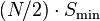, where N is the total number of drives (must be even) in the array and S_min is the capacity of the smallest drive in the array.

Six-drive RAID 0+1

Consider an example of RAID 0+1: six 120 GB drives need to be set up on a RAID 0+1. Below is an example where two 360 GB level 0 arrays are mirrored, creating 360 GB of total storage space:

Note: A1, A2, et cetera each represent one data block; each column represents one disk.

The maximum storage space here is 360 GB, spread across two arrays. The advantage is that when a hard drive fails in one of the level 0 arrays, the missing data can be transferred from the other array. However, adding an extra hard drive to one stripe requires you to add an additional hard drive to the other stripes to balance out storage among the arrays.
It is not as robust as RAID 10 and cannot tolerate two simultaneous disk failures. When 1 disk fails, the RAID 0 array that it is in will fail also. The RAID 10 array will continue to work on the remaining RAID 0 array. If a disk from that array fails before the first failing disk has been replaced, the data will be lost. That is, once a single disk fails, each of the mechanisms in the other stripe is single point of failure. Also, once the single failed mechanism is replaced, in order to rebuild its data all the disks in the array must participate in the rebuild.
The exception to this is if all the disks are hooked up to the same RAID controller in which case the controller can do the same error recovery as RAID 10 as it can still access the functional disks in each RAID 0 set. If you compare the diagrams between RAID 0+1 and RAID 10 and ignore the lines above the disks you will see that all that's different is that the disks are swapped around. If the controller has a direct link to each disk it can do the same. In this one case there is no difference between RAID 0+1 and RAID 10.
Additionally, bit error correction technologies have not kept up with rapidly rising drive capacities, resulting in higher risks of encountering media errors. In the case where a failed drive is not replaced in a RAID 0+1 configuration, a single uncorrectable media error occurring on the mirrored hard drive would result in data loss.
Given these increasing risks with RAID 0+1, many business and mission critical enterprise environments are beginning to evaluate more fault tolerant RAID setups, both RAID 10 and formats such as RAID 5 and RAID 6 that provide a smaller improvement than RAID 10 by adding underlying disk parity, but reduce overall cost. Among the more promising are hybrid approaches such as RAID 51 (mirroring above single parity) or RAID 61 (mirroring above dual parity) although neither of these delivers the reliability of the more expensive option of using RAID 10 with three way mirrors.

RAID 1 + 0

Typical RAID 1+0 setup.

A RAID 1+0, sometimes called RAID 1&0 or RAID 10, is similar to a RAID 0+1 with exception that the RAID levels used are reversed — RAID 10 is a stripe of mirrors.^[3]

Near versus far, advantages for bootable RAID

A nonstandard definition of "RAID 10" was created for the Linux MD driver^[4] ; RAID 10 as recognized by the storage industry association and as generally implemented by RAID controllers is a RAID 0 array of mirrors (which may be two way or three way mirrors) ^[5] and requires a minimum of 4 drives. Linux "RAID 10" can be implemented with as few as two disks. Implementations supporting two disks such as Linux RAID 10^[4] offer a choice of layouts, including one in which copies of a block of data are "near" each other or at the same address on different devices or predictably offset: Each disk access is split into full-speed disk accesses to different drives, yielding read and write performance like RAID 0 but without necessarily guaranteeing every stripe is on both drives. Another layout uses "a more RAID 0 like arrangement over the first half of all drives, and then a second copy in a similar layout over the second half of all drives - making sure that all copies of a block are on different drives." This has high read performance because only one of the two read locations must be found on each access, but writing requires more head seeking as two write locations must be found. Very predictable offsets minimize the seeking in either configuration. "Far" configurations may be exceptionally useful for Hybrid SSD with huge caches of 4 GB (compared to the more typical 64 MB of spinning platters in 2010) and by 2011 64 GB (as this level of storage exists now on one single chip). They may also be useful for those small pure SSD bootable RAIDs which are not reliably attached to network backup and so must maintain data for hours or days, but which are quite sensitive to the cost, power and complexity of more than two disks. Write access for SSDs is extremely fast so the multiple access become less of a problem with speed: At PCIe x4 SSD speeds, the theoretical maximum of 730 MB/s is already more than double the theoretical maximum of SATA-II at 300 MB/s.
Laptop and motherboard makers were expected to routinely include two-disk RAID 10 as options on their products by 2011^{[citation needed]} and even configure some OEM versions of operating systems with this as a default^{[citation needed]}. Among Linux users it has become extremely common.
Another use for these configurations is to continue to use slower disk interfaces in NAS or low-end RAIDs/SAS (notably SATA-II at 300 MB/s or 3 Gbit/s) rather than replace them with faster ones (USB-3 at 480 MB/s or 4.8 Gbit/s, SATA-III at 600 MB/s or 6 Gbit/s, PCIe x4 at 730 MB/s, PCIe x8 at 1460 MB/s, etc.). A pair of identical SATA-II disks with any of hybrid SSD, OS caching to a SSD or a large software write cache, could be expected to achieve performance identical to SATA-III. Three or four could achieve at least read performance similar to PCIe x8 or striped SATA-III if properly configured to minimize seek time (predictable offsets, redundant copies of most accessed data).

Examples

Note: A1, A2, et cetera each represent one data block; each column represents one disk.

More typically, larger arrays of disks are combined for professional applications. In high end configurations, enterprise storage experts expected PCIe and SAS storage to dominate and eventually replace interfaces designed for spinning metal^[6] and for these interfaces to become further integrated with Ethernet and network storage suggesting that rarely-accessed data stripes could often be located over networks and that very large arrays using protocols like iSCSI would become more common. Below is an example where three collections of 120 GB level 1 arrays are striped together to make 360 GB of total storage space:

Redundancy and data-loss recovery capability

All but one drive from each RAID 1 set could fail without damaging the data. However, if the failed drive is not replaced, the single working hard drive in the set then becomes a single point of failure for the entire array. If that single hard drive then fails, all data stored in the entire array is lost. As is the case with RAID 0+1, if a failed drive is not replaced in a RAID 10 configuration then a single uncorrectable media error occurring on the mirrored hard drive would result in data loss. Some RAID 10 vendors address this problem by supporting a "hot spare" drive, which automatically replaces and rebuilds a failed drive in the array.

Performance (speed)

According to manufacturer specifications^[7] and official independent benchmarks,^[8][9] in most cases RAID 10 provides better throughput and latency than all other RAID levels except RAID 0 (which wins in throughput).
It is the preferable RAID level for I/O-intensive applications such as database, email, and web servers, as well as for any other use requiring high disk performance.^[10]

Efficiency (potential waste of storage)

The usable capacity of a RAID 10 array is , where N is the total number of drives in the array and S_min is the capacity of the smallest drive in the array.

Implementation

The Linux kernel RAID 10 implementation (from version 2.6.9 and onwards) is not nested. The mirroring and striping is done in one process. Only certain layouts are standard RAID 10.^[4] See also the Linux MD RAID 10 and RAID 1.5 sections in the Non-standard RAID article for details.

RAID 0+3 and 3+0

This section does not cite any references or sources. Please help improve this section by adding citations to reliable sources. Unsourced material may be challenged and removed. (September 2010)

RAID 0+3

Diagram of a 0+3 array

RAID level 0+3 or RAID level 03 is a dedicated parity array across striped disks. Each block of data at the RAID 3 level is broken up amongst RAID 0 arrays where the smaller pieces are striped across disks.

RAID 30

Diagram of a 3+0 array

RAID level 30 is also known as striping of dedicated parity arrays. It is a combination of RAID level 3 and RAID level 0. RAID 30 provides high data transfer rates, combined with high data reliability. RAID 30 is best implemented on two RAID 3 disk arrays with data striped across both disk arrays. RAID 30 breaks up data into smaller blocks, and then stripes the blocks of data to each RAID 3 RAID set. RAID 3 breaks up data into smaller blocks, calculates parity by performing an Exclusive OR on the blocks, and then writes the blocks to all but one drive in the array. The parity bit created using the Exclusive OR is then written to the last drive in each RAID 3 array. The size of each block is determined by the stripe size parameter, which is set when the RAID is created.
One drive from each of the underlying RAID 3 sets can fail. Until the failed drives are replaced the other drives in the sets that suffered such a failure are a single point of failure for the entire RAID 30 array. In other words, if one of those drives fails, all data stored in the entire array is lost. The time spent in recovery (detecting and responding to a drive failure, and the rebuild process to the newly inserted drive) represents a period of vulnerability to the RAID set.

RAID 100 (RAID 1+0+0)

A RAID 100, sometimes also called RAID 10+0, is a stripe of RAID 10s. This is logically equivalent to a wider RAID 10 array, but is generally implemented using software RAID 0 over hardware RAID 10. Being "striped two ways", RAID 100 is described as a "plaid RAID".^[11] Below is an example in which two sets of two 120 GB RAID 1 arrays are striped and re-striped to make 480 GB of total storage space:

Representative RAID-100 Setup.
(Note: A1, B1, et cetera each represent one data sector; each column represents one disk.)

The failure characteristics are identical to RAID 10: all but one drive from each RAID 1 set could fail without loss of data. However, the remaining disk from the RAID 1 becomes a single point of failure for the already degraded array. Often the top level stripe is done in software. Some vendors call the top level stripe a MetaLun (Logical Unit Number (LUN)), or a Soft Stripe.
The major benefits of RAID 100 (and plaid RAID in general) over single-level RAID is spreading the load across multiple RAID controllers, giving better random read performance and mitigating hotspot risk on the array. For these reasons, RAID 100 is often the best choice for very large databases, where the hardware RAID controllers limit the number of physical disks allowed in each standard array. Implementing nested RAID levels allows virtually limitless spindle counts in a single logical volume.

RAID 50 (RAID 5+0)

Representative RAID-50 Setup.
(Note: A1, B1, et cetera each represent one data block; each column represents one disk; Ap, Bp, et cetera each represent parity information for each distinct RAID 5 and may represent different values across the RAID 5 (that is, Ap for A1 and A2 can differ from Ap for A3 and A4).)

A RAID 50 combines the straight block-level striping of RAID 0 with the distributed parity of RAID 5.^[3] This is a RAID 0 array striped across RAID 5 elements. It requires at least 6 drives.
Below is an example where three collections of 240 GB RAID 5s are striped together to make 720 GB of total storage space:
One drive from each of the RAID 5 sets could fail without loss of data. However, if the failed drive is not replaced, the remaining drives in that set then become a single point of failure for the entire array. If one of those drives fails, all data stored in the entire array is lost. The time spent in recovery (detecting and responding to a drive failure, and the rebuild process to the newly inserted drive) represents a period of vulnerability to the RAID set.
In the example below, datasets may be striped across both RAID sets. A dataset with 5 blocks would have 3 blocks written to the first RAID set, and the next 2 blocks written to RAID set 2.

RAID-50 Setup consisting of two sets of four drives each.

The configuration of the RAID sets will impact the overall fault tolerance. A construction of three seven-drive RAID 5 sets has higher capacity and storage efficiency, but can only tolerate three maximum potential drive failures. Because the reliability of the system depends on quick replacement of the bad drive so the array can rebuild, it is common to construct three six-drive RAID 5 sets each with a hot spare that can immediately start rebuilding the array on failure. This does not address the issue that the array is put under maximum strain reading every bit to rebuild the array precisely at the time when it is most vulnerable. A construction of seven three-drive RAID 5 sets can handle as many as seven drive failures but has lower capacity and storage efficiency.
RAID 50 improves upon the performance of RAID 5 particularly during writes, and provides better fault tolerance than a single RAID level does. This level is recommended for applications that require high fault tolerance, capacity and random positioning performance.
As the number of drives in a RAID set increases, and the capacity of the drives increase, this impacts the fault-recovery time correspondingly as the interval for rebuilding the RAID set increases.

RAID 51

Diagram of a RAID 51 setup.

A RAID 51 or RAID 5+1 is an array that consists of two RAID 5's that are mirrors of each other. Generally this configuration is used so that each RAID 5 resides on a separate controller. In this configuration reads and writes are balanced across both RAID 5s. Some controllers support RAID 51 across multiple channels and cards with hinting to keep the different slices synchronized. However a RAID 51 can also be accomplished using a layered RAID technique. In this configuration, the two RAID 5's have no idea that they are mirrors of each other and the RAID 1 has no idea that its underlying disks are RAID 5's. This configuration can sustain the failure of all disks in either of the arrays, plus up to one additional disk from the other array before suffering data loss. The maximum amount of space of a RAID 51 is (N) where N is the size of an individual RAID 5 set.

RAID 05 (RAID 0+5)

A RAID 0 + 5 consists of several RAID 0's (a minimum of three) that are grouped into a single RAID 5 set. The total capacity is (N-1) where N is total number of RAID 0's that make up the RAID 5. This configuration is not generally used in production systems.

RAID 53

Note that RAID 53 is typically used as a name for RAID 30 or 0+3.^[12]

RAID 60 (RAID 6+0)

A RAID 60 combines the straight block-level striping of RAID 0 with the distributed double parity of RAID 6. That is, a RAID 0 array striped across RAID 6 elements. It requires at least 8 disks.^[3]
Below is an example where two collections of 240 GB RAID 6s are striped together to make 480 GB of total storage space:

RAID-60 (RAID 6+0) Setup consisting of two sets of four drives each.

As it is based on RAID 6, two disks from each of the RAID 6 sets could fail without loss of data. Also failures while a single disk is rebuilding in one RAID 6 set will not lead to data loss. RAID 60 has improved fault tolerance, any two drives can fail without data loss and up to four total as long as it is only two from each RAID 6 sub-array.
Striping helps to increase capacity and performance without adding disks to each RAID 6 set (which would decrease data availability and could impact performance). RAID 60 improves upon the performance of RAID 6. Despite the fact that RAID 60 is slightly slower than RAID 50 in terms of writes due to the added overhead of more parity calculations, when data security is concerned this performance drop may be negligible.

Nested RAID comparison

n - Top Level Division
m - Bottom Level Division

1. ^ Delmar, Michael Graves (2003). "Data Recovery and Fault Tolerance". The Complete Guide to Networking and Network+. Cengage Learning. p. 448. ISBN 140183339X. http://books.google.com/books?id=9c1FpB8qZ8UC&dq=%22nested+raid%22&lr=&as_drrb_is=b&as_minm_is=0&as_miny_is=&as_maxm_is=0&as_maxy_is=2005&num=50&as_brr=0&source=gbs_navlinks_s. 
2. ^ Mishra, S. K.; Vemulapalli, S. K.; Mohapatra, P (1995). "Dual-Crosshatch Disk Array: A Highly Reliable Hybrid-RAID Architecture". Proceedings of the 1995 International Conference on Parallel Processing: Volume 1. CRC Press. pp. I-146ff. ISBN 084932615X. http://books.google.com/books?id=QliANH5G3_gC&dq=%22hybrid+raid%22&lr=&as_drrb_is=b&as_minm_is=0&as_miny_is=&as_maxm_is=0&as_maxy_is=1995&num=50&as_brr=0&source=gbs_navlinks_s. 
3. ^ ^{a b c d} "Selecting a RAID level and tuning performance". IBM Systems Software Information Center. IBM. 2011. p. 1. http://publib.boulder.ibm.com/infocenter/eserver/v1r2/index.jsp?topic=/diricinfo/fqy0_cselraid_copy.html. 
4. ^ ^{a b c} Brown, Neil (27 August 2004). "RAID10 in Linux MD driver". http://neil.brown.name/blog/20040827225440. 
5. ^ http://www.snia.org/tech_activities/standards/curr_standards/ddf/SNIA-DDFv1.2.pdf
6. ^ Cole, Arthur (24 August 2010). "SSDs: From SAS/SATA to PCIe". IT Business Edge. http://www.itbusinessedge.com/cm/community/features/interviews/blog/ssds-from-sassata-to-pcie/?cs=42942. 
7. ^ "Intel Rapid Storage Technology: What is RAID 10?". Intel. 16 November 2009. http://www.intel.com/support/chipsets/imsm/sb/CS-020655.htm. 
8. ^ "IBM and HP 6-Gbps SAS RAID Controller Performance" (PDF). Demartek. October 2009. http://www-03.ibm.com/systems/resources/Demartek_IBM_LSI_RAID_Controller_Performance_Evaluation_2009-10.pdf. 
9. ^ "Summary Comparison of RAID Levels". StorageReview.com. 17 May 2007. http://www.storagereview.com/guide/comp_perf_raid_levels.html. 
10. ^ Gupta, Meeta (2002). Storage Area Network Fundamentals. Cisco Press. p. 268. ISBN 1-58705-065-X. 
11. ^ McKinstry, Jim. "Server Management: Questions and Answers". Sys Admin. Archived from the original on 19 January 2008. http://web.archive.org/web/20080119125114/http://www.samag.com/documents/s=9365/sam0013h/0013h.htm. 
12. ^ Kozierok, Charles M. (17 April 2001). "RAID Levels 0+3 (03 or 53) and 3+0 (30)". The PC Guide. http://www.pcguide.com/ref/hdd/perf/raid/levels/multLevel03-c.html.